Quality Minus Junk. Asness, Cliff S. and Frazzini, Andrea and Pedersen, Lasse Heje, (June 5, 2017)

Quality companies tend to outperform junk companies, even after controlling for commonly used risk models.

0:00 - Introduction 

This paper is called "Quality Minus Junk", and it is written by Asness, Frazzini, and Pedersen.  Prior academic research has shown that companies with higher quality characteristics (e.g., lower leverage, higher profitability, lower volatility, etc.) tend to outperform those with lower quality characteristics (i.e., "junk").  As such, the authors want to explore a new factor (i.e., Quality Minus Junk) in the same way that Fama-French did with their High Minus Low, Small Minus Big, etc. factors. 

0:44 - Table 1. Summary Statistics 

The data under study includes equity securities across 24 developed markets (including the US market) over the 1957 - 2016 time period.

1:13 - Table 2. Persistence of Quality Measures 

The authors suggest that when making decisions, an investor should look to the future of the company in developing his valuations and executing his strategies.  As such, the authors want to understand whether it is possible to predict the future quality of a company.

To do that, the authors explore the persistence of quality in companies (i.e., does a company's quality today continue in the future).  They sort the US and Global stocks according to their quality ranks (including the components of safety, growth, and profitability) today, then see how those stocks rank for quality 1, 3, 5, and 10 years into the future.

They find that companies ranked high (low) in quality today tend to have high (low) quality for all time periods in the future.  As such, investors can possibly rely on the current quality of a company as a gauge for what its future quality might be.

3:24 - Table 3a. Cross Sectional Regressions, The Price of Quality 

Next, the authors want to understand whether investors pay more for higher quality companies.  To do that, they form 6 regressions on Market-to-Book ratios, with various combinations of independent variables to capture the drivers of the Market-to-Book ratios.  In all regressions, they find that a company's quality score significantly explains the Market-to-Book ratio of the companies, on average, even after controlling for several other variables; the quality score explains about 10% of the variation in Market-to-Book ratios on its own.

6:23 - Table 3b. Cross Sectional Regressions, The Price of Quality  

For this table, the authors perform the same study as in Table 3a; only this time, they split the quality score into its components: Profitability, Growth, and Safety.  They find that each of the components have merit on their own; and the overall quality score is not dominated by a single quality component.

7:18 - Table 3c. Cross Sectional Regressions, The Price of Quality  

Since prior studies have found that larger companies typically have higher quality, the authors want to understand how the price of quality is affected by company size.  To do this, the authors form the same regression as in Tables 3a and 3b; however, this time, they split the sample population into deciles of company size.  They find that the Market-to-Book ratios of larger companies (i.e., those in the higher deciles) tend to be more affected by quality scores than those of smaller companies (i.e., the coefficient on the quality factor is larger and more significant on larger companies).

8:17 - Table 4. Quality Sorted Portfolios 

Since in the prior tables we found that quality explains less than 50% of the variation in Market-to-Book ratios, the authors now want to see if there are other variables that explain the Market-to-Book ratios and whether those subsume the quality score's explanatory power.

To do so, they split the sample population into deciles according to their quality score ranks, and they find the alphas on t-bills, the CAPM model (controlling for market return), the 3-factor model (controlling for market return and value and size factors), and the 4-factor model (controlling for market return and value, size, and momentum factors).  A higher alpha on these models would lead us to conclude that there are other variables (i.e., possibly quality factors) that are not explained by the variables controlled for in each of the models.

The authors find that as the quality rank of the companies increases, the alphas and excess returns also increase after controlling for the models' factors.  The higher quality deciles also exhibit higher sharpe ratios, information ratios, and lower betas. 

12:02 - Table 5. Quality Minus Junk - Correlations  

Next, for ease of study and presentation, the authors want to determine how correlated are the components of the quality score (i.e., profitability, safety, and growth) to each other and to the overall quality score.  The authors find they are in fact highly correlated; therefore, the authors decide to scrap the individual components in the study (and only consider the overall quality score) which would ease the complexity of work on the authors and ease the presentation for their readers, without much affecting the conclusions of the study.

14:26 - Table 6. Quality Minus Junk - Returns  

Next, the authors want to explore a new factor: Quality Minus Junk (QMJ).  They build portfolios in the same way that Fama-French did with their factors: they go long the top third and short the bottom third of stocks according to their quality score ranks (also splitting into small and large in order to give fair representation to small companies).  This gives them an understanding of the returns that could be earned by investing in quality companies relative to junk companies.

The authors find a significant alpha to the QMJ portfolios after controlling for t-bills, CAPM, 3-factor, and 4-factor models.  These alphas come about because of the significantly negative relationship between the QMJ factor and the market (i.e., quality companies have lower market betas), size (i.e., quality companies tend to be larger), value (i.e., quality companies tend to be growth companies), and momentum (i.e., quality companies tend to have had a recent increase in price relative to lagging book value) factors.  As such, quality seems to be a major component/contributor to the return of each of these commonly used factors.

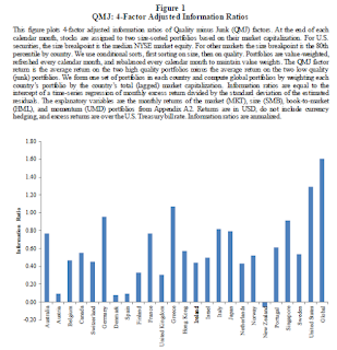
Out of all 24 countries under study, only 1 did not show a positive alpha on the 4-factor model (i.e., New Zealand, which represents the smallest market cap in the sample population).  17 of the 24 countries showed a statistically significant alpha.  As such, the efficacy of the quality factor tends to be pervasive across several markets.

17:48 - Figures 1-3. QMJ returns and alphas  

This figure shows Table 6c (discussed above) in graphical form.

This figure shows the cumulative excess returns of the QMJ portfolios over t-bills.  We see a consistently increasing and smooth accumulation.

This figure shows the cumulative alphas of the QMJ portfolios over the 4-factor model.  We see a consistently increasing and smooth accumulation.

19:09 - Table 7. 6-Factor Adjusted Returns  

Next, the authors get into robustness checks.  They perform the same study as table 6; only this time, they control for a 6-factor model (which adds the Conservative Minus Aggressive investment and Robust Minus Weak profitability) to the previous 4-factor model.  They find that the RMW factor subsumes a lot of the quality factor (which makes sense, because a component of the quality factor is profitability); and even so, a significant alpha to the QMJ portfolios is still present.

20:49 - Table 8. Returns During Different Regimes  

Next, the authors want to understand what happens with QMJ returns in different regimes (e.g., expansions and recessions, bull and bear markets, high and low volatility, etc.).  As would be expected, the QMJ portfolio performs better in bear markets than in bull markets; recessions than in expansions; and low volatility than high volatility.

22:10 - Figure 6. The Price of Quality  

Next, the authors want to understand the price of quality (i.e., how does quality affect a company's market-to-book ratio) and how it has changed over time.  They find that quality is more expensive (i.e., the market-to-book ratio increases more with increases to quality) during periods of market turmoil (such as the dot-com bubble and the housing collapse periods). 

23:51 - Table 9. Quality Sorted Portfolios - Target Prices  

Next, the authors want to understand whether an investor can buy quality at times when it is cheap, and earn excess returns to quality.  To do so, the authors sort the stocks into deciles of the quality scores and determine the price-to-book ratios, price target to book (by analysts), implied expected return, and realized 1-year return for each of the deciles.

They find that analysts typically give a higher price-to-book ratio to higher quality companies (as they should); however, relative to the current price, they are giving a lower and lower expected return to higher quality companies, while the realized 1-year returns increase as quality increases.  This presents the thought process that quality companies are currently underpriced (i.e., their current price-to-book ratio should be higher); if it were, the realized return would be more in line with analyst expectations.  As such, this scenario might give investors an opportunity to capture a return to quality.

26:03 - Equation 11. Price of Quality vs Return to Quality  

Next, the authors want to explore the possibility that lower prices to quality result in higher returns to quality.  They form a regression with the dependent variable being the return to quality and the independent variable being a lagged price of quality (and a variable to control for momentum).  If it is true that a lower price of quality results in a higher return to quality, we would expect a negative relationship between the two variables and therefore a negative coefficient on the lagged price of quality variable.

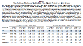
27:19 - Table 10. High Price of Quality Predicts Low QMJ Returns  

This table presents the results of the above regression.  The authors find there to be negative coefficients on the lagged price of quality variable over periods of 12, 36, and 60 months, even after controlling for t-bills and the 4-factor model.  As such, we can conclude that a lower price of quality today tends to result in a higher future return to quality.

28:46 - Table 11. Asset Pricing Test

Finally, up to this point, the QMJ has been on the left side of the regression (i.e., a dependent variable).  So now, the authors want to see what happens when QMJ is on the right side of the regression (i.e., an independent variable).  The authors find that when QMJ is added to a regression, the size factor is resurrected from insignificance.  The QMJ factor also increases the significant of the value and momentum factors by absorbing some of their explanatory power.

Suggested Citation

Asness, Cliff S. and Frazzini, Andrea and Pedersen, Lasse Heje, Quality Minus Junk (June 5, 2017). Available at SSRN: https://ssrn.com/abstract=2312432 or http://dx.doi.org/10.2139/ssrn.2312432 

Abstract

We define a quality security as one that has characteristics that, all-else-equal, an investor should be willing to pay a higher price for: stocks that are safe, profitable, growing, and well managed. High-quality stocks do have higher prices on average, but not by a very large margin. Perhaps because of this puzzlingly modest impact of quality on price, high-quality stocks have high risk-adjusted returns. Indeed, a quality-minus-junk (QMJ) factor that goes long high-quality stocks and shorts low-quality stocks earns significant risk-adjusted returns in the U.S. and globally across 24 countries. The price of quality varies over time, reaching a low during the internet bubble, and a low price of quality predicts a high future return of QMJ. Analysts’ price targets suggest that the required return of quality stock is low despite the high realized return.
 

Deep Value. Asness, Cliff S. and Liew, John M. and Pedersen, Lasse Heje and Thapar, Ashwin K (December 1, 2017)

In this paper, the authors explore the drivers and results of deep value events across several markets and asset classes.

0:00 - Introduction

Other academic studies have explored the returns to value through the construction of zero-cost portfolios (i.e., buying value stocks while shorting growth stocks).  These studies have shown significant excess returns to value that, depending on the study, have noted various risk-based and behavioral-based drivers.

In this paper called "Deep Value", by Cliff Asness and several of his colleagues at AQR Capital Management, the authors explore the returns to deep value portfolios (i.e., zero cost value portfolios occurring at times when the spread between value and growth company values are unusually large).

0:23 - Table 2. Summary Statistics and Value Performance

First, the authors provide some sample statistics and explain their methods for portfolio formation.  In their study, their data includes price/return statistics for stocks in the US, Japan, Europe, and UK markets; and index futures for equities, fixed income and currencies.  In the case of US equities, data goes back to 1926, and the other regions and asset classes generally begin in the 1970s and 1980s, ending in 2015.

For each of the asset classes and regions, the authors sort them by their Price-to-Book ratios (or the equivalent figure, in the case of non-equity asset classes) each month, and they put them into zero cost portfolios going long the top third of B/P ratios and going short the lowest third B/P ratios.  The authors also sort by B/P ratios within intra-asset classes/regions (e.g., within industries; or by pairs for non-equity asset classes).

They find in all regions and asset classes (except UK equities), the zero-cost portfolios earn a positive sharpe ratio.  These sharpe ratios are even more pronounced in intra-asset classes/regions.

 5:28 - Table 3. Value Strategy Returns by Value Spread

Next, the authors organize the zero-cost portfolios into quintiles based on their "value spread" (i.e., the difference between the book-to-price ratios of the long portion of the portfolio vs the short portion of the portfolio).  The thought is that when the value spread is larger (i.e., a "deep value" situation), we might see larger returns to value portfolios than time periods when the spread is narrower.

Indeed for all stock regions (except the UK) and asset classes, we do see increasing return as the value spread increases, monotonic increases for US equities. These are much more pronounced in the intra class portfolios.  The non-equity asset classes exhibit the same results, albeit muted.  When combining all stocks together, all non-equity asset-classes together, and all asset classes/regions together, we see monotonic increases in returns as the value spread increases.  In addition, we see significant t-statistics for the top-ranked value spread portfolios, making these results robust.

10:57 - Table 4. Value Strategy Returns Regressed on Value Spreads

Next, the authors regress the returns of the zero-cost value portfolios (i.e., the dependent variable) against the value spread (i.e., the independent variable).  They find the beta in the regression to be positive in all asset classes and regions, with significant t-statistics, giving evidence to the thought that returns to value are positively related to the value spread.

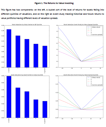
13:13 - Figure 1. The Returns to Value Investing

Next, the authors rank the stocks and non-equity asset classes by their book-to-price ratios and categorize them into quintiles based on those ranks.  They find that as the level of book-to-price ratios decrease from high (i.e., value companies) to low (i.e., growth companies), the returns of those buckets decrease monotonically, which is in line with other studies who find that value companies tend to outperform growth companies on average.

Next, the authors perform an event study that shows cumulative returns of the zero-cost portfolio in the 24 months leading up to portfolio formation and up to 24 months after portfolio formation.  They find that for all levels of value spread, the zero-cost portfolio has a negative return leading up to portfolio formation, then has positive returns up to 24 months after portfolio formation.  This means that before portfolio formation, the value (i.e., long) side of the portfolio underperforms the growth (i.e., short) side; and after portfolio formation, the value (i.e., long) side outperforms the growth (i.e., short) side.  These returns are more pronounced in deep value periods than in periods of a narrow value spread.

They performed the same analysis with non-equity asset classes (i.e., equity index, fixed income, and currency futures) as well, and find the same results.

17:36 - Figure 2. Risk Dynamics of Value Investing

Next, the authors perform the same analysis as with Figure 1, only this time they look at the market betas (rather than returns) for each B/P bucket.  They find that the market betas are near 1 for each bucket, and they slightly decrease as the buckets move from value to growth.

They also perform an event study showing the market beta of the zero cost portfolio for 2 years before to 2 years after portfolio formation.  They find that the betas (i.e., the beta of the long value side, minus the beta of the short growth side) are all below zero, signaling the zero-cost portfolio is a good hedge against market risk.  We also see that periods of deep value result in even more significantly negative betas for the zero-cost portfolio, relative to the narrow value spread periods.

Next, the authors performed the same analysis, only this time they sort the quintiles by the value betas.  As would be expected, the value portfolios load positively on the value factor and the growth portfolios load negatively on the value factor.  Also, the zero-cost portfolio (i.e., going long value stocks and short growth stocks) tends to load more on the value factor during deep value periods than during narrow value periods.  The zero-cost portfolio's loading on the value factor tends to decrease after portfolio formation as it becomes less "cheap".

The authors also perform the same analysis for non-equity asset classes and find the same results. 

21:51 - Figure 3. Earnings Fundamentals of Value

Next, the authors perform the same analysis as in figures 1 and 2, but this time they present the return-on-equity for the different value vs growth buckets.  Consistent with other research, they find the growth stocks tend to have larger returns-on-equity than do value stocks.  They also perform an event study that shows the return-on-equity for the zero-cost value portfolio 24 months before and after formation.  They find the returns-on-equity (i.e., the ROE for the long value, minus ROE for the short growth) decrease beginning 24 months before portfolio formation and continuing 24 months after portfolio formation, consistent with the idea that the ROE for growth companies exceed those of value companies.  This decrease is also more pronounced during periods of deep value than for periods of narrow value spreads.

Next, the authors perform the same analysis, only this time they present analyst earnings revisions by bucket.  They find that earnings revisions are negative for all buckets (as is consistent with the thought that analysts typically reduce earnings expectations rather than raise them); however, value companies tend to have the largest negative earnings revisions compared to growth companies.  This is also evident in the event study which shows the earnings revisions of value minus the earnings revisions of growth stocks to decrease over time; this trend does seem to reverse a year after formation, however.  Deep value events tend to exacerbate these results compared to narrow value spread events.

24:25 - Figure 4. News Sentiment of Value 

Next, the same analysis as figures 1, 2, and 3 is performed, only this time the authors look at news sentiment across the different value/growth buckets and over the -2/+2 year event horizon.  They find that growth companies tend to have more positive news sentiment than do value companies.  During the 2 years leading up to the zero-cost value portfolio formation, the sentiment for growth stocks exceeds that of value stocks; however, in the 2 years after formation, the sentiment for value stocks exceeds that of growth stocks.  Deeper value time periods show more extreme differences in sentiment between value and growth than do more narrow value spread periods.

26:02 - Figure 5. Demand Pressure

Next, the authors perform the same analysis as figures 1-4, only this time they look at demand pressure for value vs growth stocks (i.e., dollar buys, less dollar sells for stocks).  They find that growth stocks tend to be more in demand than value companies.  As a result of this, the cumulative difference between demand for the value side and the growth side of the demand pressure decreases over the 4 year event horizon; this difference tends to be more pronounced for deep value periods as opposed to narrow value spread time periods.

27:19 - Table 5. What Do Investors (Over-)React To

Next, the authors explore the drivers of the demand pressure and returns to zero-cost value portfolios, by regressing each of these against past returns and past return on equity.

They find the demand pressure is positively related to the past returns and past ROE; however, the ROE factor is subsumed by the past returns when combined in a regression.  This signals that past returns and past ROE or correlated, and confirms prior studies that suggest investors over-extrapolate past returns when making investment decisions.

They also find the 1-month returns are positively related to 1-year past returns and negatively related to 5-year past returns, confirming prior studies that suggest investors over-react to past short-term returns, which results in initial momentum and a reversal later on.  The authors also find that when controlling for past returns, the past ROE is positively related to the 1-month returns; this might suggest that investors under-react to fundamental information, consistent with other studies.

30:27 - Figure 6. The Limits of Value Arbitrage

Next, the authors explore a few costs or hindrances to value arbitrageurs, which might be contributing to the persistence of value returns.

First, they find that bid-ask spreads for value companies tend to be much larger than those for growth companies.  These bid-ask spreads for implementing the zero-cost value portfolio are more pronounced during deep value periods as opposed to narrow value spread periods.

Next, they find that short fees (i.e., the cost of shorting the growth side in the zero-cost portfolio) are expensive for both value and growth companies, but not so much for the interior buckets.  Looking at the growth side only (because that's the side that is being shorted in the zero-cost portfolio), they find the short fees are much higher during periods of deep value as opposed to periods of narrow value spreads.

Finally, the authors find that value stocks tend to be more volatile than growth stocks.  In addition, the volatility of the zero-cost portfolio is much higher during deep value periods compared to narrow value spread periods.

These higher bid-ask spreads, higher short fees, and higher volatility all present larger costs and risks to a value arbitrageur, therefore contributing to the persistence of excess value returns.

33:27 - Figure 7. Value Arbitrage Activity

Next, the authors explore whether investors (i.e., by shorting growth companies), the value companies themselves (i.e., through share buy-backs) or acquirers (i.e., by acquiring value companies) might be the value arbitrageurs.

First, they look at short-interest for the different buckets of value vs growth stocks.  They find no meaningful difference between the short interest of growth companies than value companies. There is also not a meaningful change in short interest for growth companies over the 4 year event horizon; although, there is a dip around the portfolio formation time period possibly signaling investors' capital problems as growth stock prices are increasing as their short positions falter.  There is much larger short interest for growth companies during deep value events as opposed to those of narrow value spread periods.

Next, the authors explore the difference in stock buy-backs for value vs growth companies, in an effort to determine whether the companies themselves are arbitraging their stock values that they perceive as cheap.  They find that growth companies tend to issue more shares relative to value companies, although value companies still tend to issue more shares than they buy back.  When exploring the buy-backs of the value companies minus the buy-backs of the growth companies, they find that after portfolio formation date, the value companies are buying back more shares than are the growth companies.  This result is more pronounced for deep value periods compared to narrow value spread periods.

Finally, the authors explore whether acquirers are buying value companies when they get cheap.  They find that value companies are acquired more often than are growth companies.  They also find that the difference between the acquisition of value companies vs the acquisition of growth companies increases for the next two years after formation date; and this result is more pronounced for deep value periods compared to narrow spread periods.

All of this suggests that investors, the companies themselves, and acquirers are doing their part to arbitrage away the mispricing of value vs growth stocks; and these opportunities are taken advantage of more often when the value spreads get extremely deep.

37:21 - Table 6. The Alpha of Deep Value Out-of-Sample

Next, the authors explore out-of-sample tests for all 4 equity markets and all 3 asset classes to see what would the returns and characteristics of those returns have been under various trading strategies.  First, they developed a trading strategy of buying into the zero-cost value portfolio (i.e., go long value companies and short growth companies) when the value spread (i.e., the spread between the B/P ratio of the value companies and the B/P ratio of the growth companies) exceeds its 80th percentile of data to that point; and exiting the zero-cost value portfolio when the value spread goes back below its median.

For each of the individual markets or asset classes, they find that the returns load significantly positively on the global value factor and significantly negatively on the momentum factor, with no significant loading on alpha (i.e., timing the value factor doesn't necessarily result in better performance than a passive value strategy).  However, when all markets and asset classes are combined, they find a significant alpha figure.

The authors also perform this analysis for the intra-portfolios as well and find similar results, albeit with even more significant alphas. 

39:51 - Table 7. The Alpha of Deep Value Out-of-Sample: Robustness

Next, the authors explore different trading strategies similar to the one in Table 6.  They implement a "deep value" strategy (i.e., in at 80th percentile, out at median), "deeper value" strategy (i.e., in at 2 standard deviations, out at 1 standard deviation), "threshold" strategy (i.e., in at 80th percentile, out at 80th percentile), and "linear" strategy (i.e., allocation in proportion to the value spread level).  They find that the "deeper value" strategy performs slightly better (i.e., it has a higher alpha) than the "deep value" strategy, and significantly better than the others; however, the results are similar across all strategies, where there are significant positive loadings to the value factor and alpha and a significant negative loading to the momentum factor.  The intra-portfolios have similar results.

42:00 - Figure 8. Deep Value Strategy Cumulative Returns and Opportunity Set

Next the authors quantify and chart the cumulative returns to the "deep value" strategy as well as the opportunity set (i.e., the number of times the portfolios are in a "deep value" situation).  They find deep value events clustered around significant world/US events, such as the 2001 and 2008 recessions, Iraq War in the early 90s, and Volker experiments.  They also find significant and positive returns during the deep value event periods and across the entire sample period.

42:59 - Table 8. Deep Value Returns Vs The Number of Deep Value Opportunities

Finally, the authors developed a regression of returns, volatility, and sharpe ratios of the deep value portfolios against the size of the opportunity set.  They find that the larger the opportunity set of deep value event periods, the higher the return, volatility, and sharpe ratios of the deep value strategy.

Abstract

We define “deep value” as episodes where the valuation spread between cheap and expensive securities is wide relative to its history. Examining deep value across global individual equities, equity index futures, currencies, and global bonds provides new evidence on competing theories for the value premium.

Following these episodes, the value strategy has:

(1) high average returns;
(2) low market betas, but high betas to a global value factor;
(3) deteriorating fundamentals;
(4) negative news sentiment;
(5) selling pressure;
(6) increased limits to arbitrage; and
(7) increased arbitrage activity.

Lastly, we find that deep value episodes tend to cluster and a deep value trading strategy generates excess returns not explained by traditional risk factors.


Suggested Citation:
Asness, Cliff S. and Liew, John M. and Pedersen, Lasse Heje and Thapar, Ashwin K, Deep Value (December 1, 2017). Available at SSRN: https://ssrn.com/abstract=3076181 or http://dx.doi.org/10.2139/ssrn.3076181

A tale of two states: asymmetries in the UK small, value and momentum premiums. Sarwar et al (2017)

The authors are looking to explore the style premiums in the UK over the 1982 - 2014 period.  They also want to explore how the premiums are affected by various macroeconomic indicators in expansionary and recessionary regimes. 

First, they look at the size, value, and momentum premiums over the full period and find the momentum period to be 0.95%, followed by the value premium at 0.34%, and finally the size premium at 0.12%.  Next, they split the sample into expansion and recession regimes and find that the value and momentum premiums remain the same no matter if in an expansionary or recessionary regime; however, they find that the size premium actually goes negative during a recession.  They also find that the size premium is positively skewed, while the value and momentum premiums are negatively skewed, no matter the regime.

Next, the authors regress various macroeconomic indicators against the size, value, and momentum factor premiums.  They find that increases to the GDP growth rate, inflation, and money supply significantly explain increases to the size premium; increases to the short-term interest rates and credit spread significantly explain an increase to the value premium; and no macroeconomic indicators significantly explain the changes in the momentum premium.   However, the R^2 of the regressions are very small, so the regression equation likely does not provide a good enough fit.

Next, the authors split that sample into two regimes: expansion and recession; where they regress the same macroeconomic indicators against the same factor premiums in the two different regimes.  They find that the alphas in the regression equation are negative for the size and value premiums, so investors are likely better off owning large-gap growth companies during a recession; also, the factor premium for momentum is significantly less during a recession than in an expansion. 

An increase to the GDP growth rate positively explains the size and value premiums in an expansion; however, it negatively explains the value premium in a recession.  The authors suggest that value companies tend to be in certain industries that don't turn around until late in the economic cycle, thereby foregoing the benefits of GDP growth during the recession.

An increase to inflation positively explains the size premium in both regimes, but is insignificant for the other factors.  The authors suggest that it's easier for smaller companies to pass along price increases, so they would maintain their profitability.

An increase to the short-term interest rates positively explains the size premium in a recession; the authors suggest that small companies have a more difficult time obtaining capital, so an increase to interest rates hurts them more than large companies, and they therefore earn a premium for that risk.  An increase to short-term interest rates positively explains the value premium in both regimes; the authors suggest that value companies are much more leveraged than growth companies, and investors would require a higher premium over growth companies for taking on that risk during a rising rate environment.  An increase to short-term interest rates negatively explains the momentum premium in both regimes.

An increase to the term structure positively explains the size premium in a recession.  An increase to the term structure positively explains the value premium in an expansion and negatively explains the value premium in a recession; the authors suggest that growth companies don't pay as high a dividend, so when the credit spread increase, the investors require a higher premium to compensate them for the higher rate environment that they are foregoing.  An increase in the term structure negatively explains the momentum premium in a recession; the authors suggest that the past winner are typically higher beta, so as the term spread increases, the market price goes down and more severely affects the higher beta companies than the lower beta companies.

An increase to the credit spread positively affects the size and value premiums in both regimes.  An increase to the credit spread negatively affects the momentum premium in an expansion and positively affects the momentum premium in a recession.

An increase to the money supply does not significantly affect any of the factors in an expansion; however, it is positively related to the size factor and negatively related to the value factor in a recession.  The authors suggest that smaller companies do not have as easy access to the growth in the money supply that bigger companies do, so investors require a higher premium for not being relieved from the ongoing recession.

Sarwar, G., Mateus, C., & Todorovic, N. (2017). A tale of two states: asymmetries in the UK small, value and momentum premiums. Applied Economics, 49(5), 456–476.

Alphas in disguise: A new approach to uncovering them

The Carhart 4-factor model has become the academic standard for explaining returns; however, recently passive indices have been shown to have non-zero alphas in their 4-factor models, which should not be so for passive indices that represent the market.  Either the wrong factors are being selected or there are errors in the calculations of those factors used. 

Previous studies have suggested that one error may be the SMB calculation: some small funds may actually have big companies in them, because, since big companies are small relative to the whole market, causing a biased positive SMB estimate.  This goes for the other winner/loser, value/growth factors as well.  To mitigate that error, other studies have reduced alpha in indices by including only only US Equities in the market portfolio, make the HML and SMB portfolios be value-weighted instead of equal-weighted, separate value/growth stocks and small/big stocks, and make the sizes more granular (such as large-cap, mid-cap, small-cap, etc.).

The authors study 1,383 US equity mutual funds over the period January 1992 to October 2013, who designate the S&P 500 as their benchmark.  They then make adjustments to the Carhart 4-factors (obtained from Ken French's website) that will bring the alpha to zero.  In their calculations, they find both active and passive funds perform worse on an adjusted alpha basis than what is implied by the unadjusted Carhart 4-factor model. 

Also noted is that the passive tracker funds performed the worst over the period, showing significant negative alphas; which is counter-intuitive, considering a passive tracker fund should have a zero alpha.  Active mutual funds perform outperform in some periods and under-perform in others.

Chinthalapati, V., Mateus, C., & Todorovic, N. (2017). Alphas in disguise: A new approach to uncovering them. International Journal of Finance & Economics, 22(3), 234–243.

A tale of two states: asymmetries in the UK small, value and momentum premiums

The authors study the asymmetries in the value, size, and momentum factor premiums across expansionary and recessionary regimes in the UK over the period January 1982 - June 2014.  They find strong evidence for asymmetries across all three factors in the different regimes; the size premium showed the strongest asymmetry (even turning negative in the recessionary regime), and the momentum factor showed the least asymmetry.

The authors also corroborate US studies by finding that macroeconomic factors (such as GDP Growth, credit, inflation, etc.) are significant determinants of value/size/momentum factor premiums, especially in market downturns.  The authors also developed a Markov switching model and back-tested a portfolio, beating a buy and hold strategy across  8 size/value/momentum portfolios.

Sarwar, G., Mateus, C., & Todorovic, N. (2017). A tale of two states: asymmetries in the UK small, value and momentum premiums. Applied Economics, 49(5), 456–476.

Size, Value, Momentum in Indian Equities

The authors study the Indian equity markets during the period January 1994 - March 2017.  In doing so they seek to learn the performance of the value (HML), size (SMB), and momentum indicators (12-1) in that market over that time period.

They used the Fama-French methodology to form portfolios and determined that value significantly outperformed growth and winners significantly outperformed losers; however, small cap significantly underperformed large cap, which is contrary to the Fama French and other studies.

The HML factor returned 9.08% with an annualized volatility of 16.33%, and a max draw-down of 53%.  The size factor returned 0.36% with an annualized volatility of 14.51% and a max drawdown of 74% in 1995 that never recovered.  The momentum factor returned 17.3% with an annualized volatility of 17.06%, and a max draw-down of 49%.

The authors further mean-variance optimized the factors with market factors and a risk-free rate; interestingly, the portfolios at moderate/high risk levels primarily held momentum and value factors, while lower risk portfolios primarily held the risk-free security.  The market factor was a small weight in all portfolios.


Agarwalla, S. K., Jacob, J., & Varma, J. R. (2017). Size, Value, and Momentum in Indian Equities. Vikalpa: The Journal for Decision Makers, 42(4), 211–219.