Quality Minus Junk. Asness, Cliff S. and Frazzini, Andrea and Pedersen, Lasse Heje, (June 5, 2017)

Quality companies tend to outperform junk companies, even after controlling for commonly used risk models.

0:00 - Introduction 

This paper is called "Quality Minus Junk", and it is written by Asness, Frazzini, and Pedersen.  Prior academic research has shown that companies with higher quality characteristics (e.g., lower leverage, higher profitability, lower volatility, etc.) tend to outperform those with lower quality characteristics (i.e., "junk").  As such, the authors want to explore a new factor (i.e., Quality Minus Junk) in the same way that Fama-French did with their High Minus Low, Small Minus Big, etc. factors. 

0:44 - Table 1. Summary Statistics 

The data under study includes equity securities across 24 developed markets (including the US market) over the 1957 - 2016 time period.

1:13 - Table 2. Persistence of Quality Measures 

The authors suggest that when making decisions, an investor should look to the future of the company in developing his valuations and executing his strategies.  As such, the authors want to understand whether it is possible to predict the future quality of a company.

To do that, the authors explore the persistence of quality in companies (i.e., does a company's quality today continue in the future).  They sort the US and Global stocks according to their quality ranks (including the components of safety, growth, and profitability) today, then see how those stocks rank for quality 1, 3, 5, and 10 years into the future.

They find that companies ranked high (low) in quality today tend to have high (low) quality for all time periods in the future.  As such, investors can possibly rely on the current quality of a company as a gauge for what its future quality might be.

3:24 - Table 3a. Cross Sectional Regressions, The Price of Quality 

Next, the authors want to understand whether investors pay more for higher quality companies.  To do that, they form 6 regressions on Market-to-Book ratios, with various combinations of independent variables to capture the drivers of the Market-to-Book ratios.  In all regressions, they find that a company's quality score significantly explains the Market-to-Book ratio of the companies, on average, even after controlling for several other variables; the quality score explains about 10% of the variation in Market-to-Book ratios on its own.

6:23 - Table 3b. Cross Sectional Regressions, The Price of Quality  

For this table, the authors perform the same study as in Table 3a; only this time, they split the quality score into its components: Profitability, Growth, and Safety.  They find that each of the components have merit on their own; and the overall quality score is not dominated by a single quality component.

7:18 - Table 3c. Cross Sectional Regressions, The Price of Quality  

Since prior studies have found that larger companies typically have higher quality, the authors want to understand how the price of quality is affected by company size.  To do this, the authors form the same regression as in Tables 3a and 3b; however, this time, they split the sample population into deciles of company size.  They find that the Market-to-Book ratios of larger companies (i.e., those in the higher deciles) tend to be more affected by quality scores than those of smaller companies (i.e., the coefficient on the quality factor is larger and more significant on larger companies).

8:17 - Table 4. Quality Sorted Portfolios 

Since in the prior tables we found that quality explains less than 50% of the variation in Market-to-Book ratios, the authors now want to see if there are other variables that explain the Market-to-Book ratios and whether those subsume the quality score's explanatory power.

To do so, they split the sample population into deciles according to their quality score ranks, and they find the alphas on t-bills, the CAPM model (controlling for market return), the 3-factor model (controlling for market return and value and size factors), and the 4-factor model (controlling for market return and value, size, and momentum factors).  A higher alpha on these models would lead us to conclude that there are other variables (i.e., possibly quality factors) that are not explained by the variables controlled for in each of the models.

The authors find that as the quality rank of the companies increases, the alphas and excess returns also increase after controlling for the models' factors.  The higher quality deciles also exhibit higher sharpe ratios, information ratios, and lower betas. 

12:02 - Table 5. Quality Minus Junk - Correlations  

Next, for ease of study and presentation, the authors want to determine how correlated are the components of the quality score (i.e., profitability, safety, and growth) to each other and to the overall quality score.  The authors find they are in fact highly correlated; therefore, the authors decide to scrap the individual components in the study (and only consider the overall quality score) which would ease the complexity of work on the authors and ease the presentation for their readers, without much affecting the conclusions of the study.

14:26 - Table 6. Quality Minus Junk - Returns  

Next, the authors want to explore a new factor: Quality Minus Junk (QMJ).  They build portfolios in the same way that Fama-French did with their factors: they go long the top third and short the bottom third of stocks according to their quality score ranks (also splitting into small and large in order to give fair representation to small companies).  This gives them an understanding of the returns that could be earned by investing in quality companies relative to junk companies.

The authors find a significant alpha to the QMJ portfolios after controlling for t-bills, CAPM, 3-factor, and 4-factor models.  These alphas come about because of the significantly negative relationship between the QMJ factor and the market (i.e., quality companies have lower market betas), size (i.e., quality companies tend to be larger), value (i.e., quality companies tend to be growth companies), and momentum (i.e., quality companies tend to have had a recent increase in price relative to lagging book value) factors.  As such, quality seems to be a major component/contributor to the return of each of these commonly used factors.

Out of all 24 countries under study, only 1 did not show a positive alpha on the 4-factor model (i.e., New Zealand, which represents the smallest market cap in the sample population).  17 of the 24 countries showed a statistically significant alpha.  As such, the efficacy of the quality factor tends to be pervasive across several markets.

17:48 - Figures 1-3. QMJ returns and alphas  

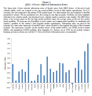
This figure shows Table 6c (discussed above) in graphical form.

This figure shows the cumulative excess returns of the QMJ portfolios over t-bills.  We see a consistently increasing and smooth accumulation.

This figure shows the cumulative alphas of the QMJ portfolios over the 4-factor model.  We see a consistently increasing and smooth accumulation.

19:09 - Table 7. 6-Factor Adjusted Returns  

Next, the authors get into robustness checks.  They perform the same study as table 6; only this time, they control for a 6-factor model (which adds the Conservative Minus Aggressive investment and Robust Minus Weak profitability) to the previous 4-factor model.  They find that the RMW factor subsumes a lot of the quality factor (which makes sense, because a component of the quality factor is profitability); and even so, a significant alpha to the QMJ portfolios is still present.

20:49 - Table 8. Returns During Different Regimes  

Next, the authors want to understand what happens with QMJ returns in different regimes (e.g., expansions and recessions, bull and bear markets, high and low volatility, etc.).  As would be expected, the QMJ portfolio performs better in bear markets than in bull markets; recessions than in expansions; and low volatility than high volatility.

22:10 - Figure 6. The Price of Quality  

Next, the authors want to understand the price of quality (i.e., how does quality affect a company's market-to-book ratio) and how it has changed over time.  They find that quality is more expensive (i.e., the market-to-book ratio increases more with increases to quality) during periods of market turmoil (such as the dot-com bubble and the housing collapse periods). 

23:51 - Table 9. Quality Sorted Portfolios - Target Prices  

Next, the authors want to understand whether an investor can buy quality at times when it is cheap, and earn excess returns to quality.  To do so, the authors sort the stocks into deciles of the quality scores and determine the price-to-book ratios, price target to book (by analysts), implied expected return, and realized 1-year return for each of the deciles.

They find that analysts typically give a higher price-to-book ratio to higher quality companies (as they should); however, relative to the current price, they are giving a lower and lower expected return to higher quality companies, while the realized 1-year returns increase as quality increases.  This presents the thought process that quality companies are currently underpriced (i.e., their current price-to-book ratio should be higher); if it were, the realized return would be more in line with analyst expectations.  As such, this scenario might give investors an opportunity to capture a return to quality.

26:03 - Equation 11. Price of Quality vs Return to Quality  

Next, the authors want to explore the possibility that lower prices to quality result in higher returns to quality.  They form a regression with the dependent variable being the return to quality and the independent variable being a lagged price of quality (and a variable to control for momentum).  If it is true that a lower price of quality results in a higher return to quality, we would expect a negative relationship between the two variables and therefore a negative coefficient on the lagged price of quality variable.

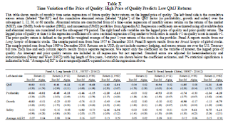
27:19 - Table 10. High Price of Quality Predicts Low QMJ Returns  

This table presents the results of the above regression.  The authors find there to be negative coefficients on the lagged price of quality variable over periods of 12, 36, and 60 months, even after controlling for t-bills and the 4-factor model.  As such, we can conclude that a lower price of quality today tends to result in a higher future return to quality.

28:46 - Table 11. Asset Pricing Test

Finally, up to this point, the QMJ has been on the left side of the regression (i.e., a dependent variable).  So now, the authors want to see what happens when QMJ is on the right side of the regression (i.e., an independent variable).  The authors find that when QMJ is added to a regression, the size factor is resurrected from insignificance.  The QMJ factor also increases the significant of the value and momentum factors by absorbing some of their explanatory power.

Suggested Citation

Asness, Cliff S. and Frazzini, Andrea and Pedersen, Lasse Heje, Quality Minus Junk (June 5, 2017). Available at SSRN: https://ssrn.com/abstract=2312432 or http://dx.doi.org/10.2139/ssrn.2312432 

Abstract

We define a quality security as one that has characteristics that, all-else-equal, an investor should be willing to pay a higher price for: stocks that are safe, profitable, growing, and well managed. High-quality stocks do have higher prices on average, but not by a very large margin. Perhaps because of this puzzlingly modest impact of quality on price, high-quality stocks have high risk-adjusted returns. Indeed, a quality-minus-junk (QMJ) factor that goes long high-quality stocks and shorts low-quality stocks earns significant risk-adjusted returns in the U.S. and globally across 24 countries. The price of quality varies over time, reaching a low during the internet bubble, and a low price of quality predicts a high future return of QMJ. Analysts’ price targets suggest that the required return of quality stock is low despite the high realized return.
 

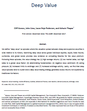
Deep Value. Asness, Cliff S. and Liew, John M. and Pedersen, Lasse Heje and Thapar, Ashwin K (December 1, 2017)

In this paper, the authors explore the drivers and results of deep value events across several markets and asset classes.

0:00 - Introduction

Other academic studies have explored the returns to value through the construction of zero-cost portfolios (i.e., buying value stocks while shorting growth stocks).  These studies have shown significant excess returns to value that, depending on the study, have noted various risk-based and behavioral-based drivers.

In this paper called "Deep Value", by Cliff Asness and several of his colleagues at AQR Capital Management, the authors explore the returns to deep value portfolios (i.e., zero cost value portfolios occurring at times when the spread between value and growth company values are unusually large).

0:23 - Table 2. Summary Statistics and Value Performance

First, the authors provide some sample statistics and explain their methods for portfolio formation.  In their study, their data includes price/return statistics for stocks in the US, Japan, Europe, and UK markets; and index futures for equities, fixed income and currencies.  In the case of US equities, data goes back to 1926, and the other regions and asset classes generally begin in the 1970s and 1980s, ending in 2015.

For each of the asset classes and regions, the authors sort them by their Price-to-Book ratios (or the equivalent figure, in the case of non-equity asset classes) each month, and they put them into zero cost portfolios going long the top third of B/P ratios and going short the lowest third B/P ratios.  The authors also sort by B/P ratios within intra-asset classes/regions (e.g., within industries; or by pairs for non-equity asset classes).

They find in all regions and asset classes (except UK equities), the zero-cost portfolios earn a positive sharpe ratio.  These sharpe ratios are even more pronounced in intra-asset classes/regions.

 5:28 - Table 3. Value Strategy Returns by Value Spread

Next, the authors organize the zero-cost portfolios into quintiles based on their "value spread" (i.e., the difference between the book-to-price ratios of the long portion of the portfolio vs the short portion of the portfolio).  The thought is that when the value spread is larger (i.e., a "deep value" situation), we might see larger returns to value portfolios than time periods when the spread is narrower.

Indeed for all stock regions (except the UK) and asset classes, we do see increasing return as the value spread increases, monotonic increases for US equities. These are much more pronounced in the intra class portfolios.  The non-equity asset classes exhibit the same results, albeit muted.  When combining all stocks together, all non-equity asset-classes together, and all asset classes/regions together, we see monotonic increases in returns as the value spread increases.  In addition, we see significant t-statistics for the top-ranked value spread portfolios, making these results robust.

10:57 - Table 4. Value Strategy Returns Regressed on Value Spreads

Next, the authors regress the returns of the zero-cost value portfolios (i.e., the dependent variable) against the value spread (i.e., the independent variable).  They find the beta in the regression to be positive in all asset classes and regions, with significant t-statistics, giving evidence to the thought that returns to value are positively related to the value spread.

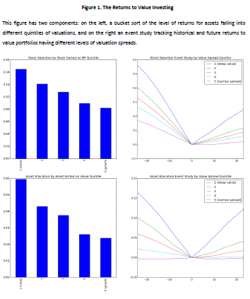
13:13 - Figure 1. The Returns to Value Investing

Next, the authors rank the stocks and non-equity asset classes by their book-to-price ratios and categorize them into quintiles based on those ranks.  They find that as the level of book-to-price ratios decrease from high (i.e., value companies) to low (i.e., growth companies), the returns of those buckets decrease monotonically, which is in line with other studies who find that value companies tend to outperform growth companies on average.

Next, the authors perform an event study that shows cumulative returns of the zero-cost portfolio in the 24 months leading up to portfolio formation and up to 24 months after portfolio formation.  They find that for all levels of value spread, the zero-cost portfolio has a negative return leading up to portfolio formation, then has positive returns up to 24 months after portfolio formation.  This means that before portfolio formation, the value (i.e., long) side of the portfolio underperforms the growth (i.e., short) side; and after portfolio formation, the value (i.e., long) side outperforms the growth (i.e., short) side.  These returns are more pronounced in deep value periods than in periods of a narrow value spread.

They performed the same analysis with non-equity asset classes (i.e., equity index, fixed income, and currency futures) as well, and find the same results.

17:36 - Figure 2. Risk Dynamics of Value Investing

Next, the authors perform the same analysis as with Figure 1, only this time they look at the market betas (rather than returns) for each B/P bucket.  They find that the market betas are near 1 for each bucket, and they slightly decrease as the buckets move from value to growth.

They also perform an event study showing the market beta of the zero cost portfolio for 2 years before to 2 years after portfolio formation.  They find that the betas (i.e., the beta of the long value side, minus the beta of the short growth side) are all below zero, signaling the zero-cost portfolio is a good hedge against market risk.  We also see that periods of deep value result in even more significantly negative betas for the zero-cost portfolio, relative to the narrow value spread periods.

Next, the authors performed the same analysis, only this time they sort the quintiles by the value betas.  As would be expected, the value portfolios load positively on the value factor and the growth portfolios load negatively on the value factor.  Also, the zero-cost portfolio (i.e., going long value stocks and short growth stocks) tends to load more on the value factor during deep value periods than during narrow value periods.  The zero-cost portfolio's loading on the value factor tends to decrease after portfolio formation as it becomes less "cheap".

The authors also perform the same analysis for non-equity asset classes and find the same results. 

21:51 - Figure 3. Earnings Fundamentals of Value

Next, the authors perform the same analysis as in figures 1 and 2, but this time they present the return-on-equity for the different value vs growth buckets.  Consistent with other research, they find the growth stocks tend to have larger returns-on-equity than do value stocks.  They also perform an event study that shows the return-on-equity for the zero-cost value portfolio 24 months before and after formation.  They find the returns-on-equity (i.e., the ROE for the long value, minus ROE for the short growth) decrease beginning 24 months before portfolio formation and continuing 24 months after portfolio formation, consistent with the idea that the ROE for growth companies exceed those of value companies.  This decrease is also more pronounced during periods of deep value than for periods of narrow value spreads.

Next, the authors perform the same analysis, only this time they present analyst earnings revisions by bucket.  They find that earnings revisions are negative for all buckets (as is consistent with the thought that analysts typically reduce earnings expectations rather than raise them); however, value companies tend to have the largest negative earnings revisions compared to growth companies.  This is also evident in the event study which shows the earnings revisions of value minus the earnings revisions of growth stocks to decrease over time; this trend does seem to reverse a year after formation, however.  Deep value events tend to exacerbate these results compared to narrow value spread events.

24:25 - Figure 4. News Sentiment of Value 

Next, the same analysis as figures 1, 2, and 3 is performed, only this time the authors look at news sentiment across the different value/growth buckets and over the -2/+2 year event horizon.  They find that growth companies tend to have more positive news sentiment than do value companies.  During the 2 years leading up to the zero-cost value portfolio formation, the sentiment for growth stocks exceeds that of value stocks; however, in the 2 years after formation, the sentiment for value stocks exceeds that of growth stocks.  Deeper value time periods show more extreme differences in sentiment between value and growth than do more narrow value spread periods.

26:02 - Figure 5. Demand Pressure

Next, the authors perform the same analysis as figures 1-4, only this time they look at demand pressure for value vs growth stocks (i.e., dollar buys, less dollar sells for stocks).  They find that growth stocks tend to be more in demand than value companies.  As a result of this, the cumulative difference between demand for the value side and the growth side of the demand pressure decreases over the 4 year event horizon; this difference tends to be more pronounced for deep value periods as opposed to narrow value spread time periods.

27:19 - Table 5. What Do Investors (Over-)React To

Next, the authors explore the drivers of the demand pressure and returns to zero-cost value portfolios, by regressing each of these against past returns and past return on equity.

They find the demand pressure is positively related to the past returns and past ROE; however, the ROE factor is subsumed by the past returns when combined in a regression.  This signals that past returns and past ROE or correlated, and confirms prior studies that suggest investors over-extrapolate past returns when making investment decisions.

They also find the 1-month returns are positively related to 1-year past returns and negatively related to 5-year past returns, confirming prior studies that suggest investors over-react to past short-term returns, which results in initial momentum and a reversal later on.  The authors also find that when controlling for past returns, the past ROE is positively related to the 1-month returns; this might suggest that investors under-react to fundamental information, consistent with other studies.

30:27 - Figure 6. The Limits of Value Arbitrage

Next, the authors explore a few costs or hindrances to value arbitrageurs, which might be contributing to the persistence of value returns.

First, they find that bid-ask spreads for value companies tend to be much larger than those for growth companies.  These bid-ask spreads for implementing the zero-cost value portfolio are more pronounced during deep value periods as opposed to narrow value spread periods.

Next, they find that short fees (i.e., the cost of shorting the growth side in the zero-cost portfolio) are expensive for both value and growth companies, but not so much for the interior buckets.  Looking at the growth side only (because that's the side that is being shorted in the zero-cost portfolio), they find the short fees are much higher during periods of deep value as opposed to periods of narrow value spreads.

Finally, the authors find that value stocks tend to be more volatile than growth stocks.  In addition, the volatility of the zero-cost portfolio is much higher during deep value periods compared to narrow value spread periods.

These higher bid-ask spreads, higher short fees, and higher volatility all present larger costs and risks to a value arbitrageur, therefore contributing to the persistence of excess value returns.

33:27 - Figure 7. Value Arbitrage Activity

Next, the authors explore whether investors (i.e., by shorting growth companies), the value companies themselves (i.e., through share buy-backs) or acquirers (i.e., by acquiring value companies) might be the value arbitrageurs.

First, they look at short-interest for the different buckets of value vs growth stocks.  They find no meaningful difference between the short interest of growth companies than value companies. There is also not a meaningful change in short interest for growth companies over the 4 year event horizon; although, there is a dip around the portfolio formation time period possibly signaling investors' capital problems as growth stock prices are increasing as their short positions falter.  There is much larger short interest for growth companies during deep value events as opposed to those of narrow value spread periods.

Next, the authors explore the difference in stock buy-backs for value vs growth companies, in an effort to determine whether the companies themselves are arbitraging their stock values that they perceive as cheap.  They find that growth companies tend to issue more shares relative to value companies, although value companies still tend to issue more shares than they buy back.  When exploring the buy-backs of the value companies minus the buy-backs of the growth companies, they find that after portfolio formation date, the value companies are buying back more shares than are the growth companies.  This result is more pronounced for deep value periods compared to narrow value spread periods.

Finally, the authors explore whether acquirers are buying value companies when they get cheap.  They find that value companies are acquired more often than are growth companies.  They also find that the difference between the acquisition of value companies vs the acquisition of growth companies increases for the next two years after formation date; and this result is more pronounced for deep value periods compared to narrow spread periods.

All of this suggests that investors, the companies themselves, and acquirers are doing their part to arbitrage away the mispricing of value vs growth stocks; and these opportunities are taken advantage of more often when the value spreads get extremely deep.

37:21 - Table 6. The Alpha of Deep Value Out-of-Sample

Next, the authors explore out-of-sample tests for all 4 equity markets and all 3 asset classes to see what would the returns and characteristics of those returns have been under various trading strategies.  First, they developed a trading strategy of buying into the zero-cost value portfolio (i.e., go long value companies and short growth companies) when the value spread (i.e., the spread between the B/P ratio of the value companies and the B/P ratio of the growth companies) exceeds its 80th percentile of data to that point; and exiting the zero-cost value portfolio when the value spread goes back below its median.

For each of the individual markets or asset classes, they find that the returns load significantly positively on the global value factor and significantly negatively on the momentum factor, with no significant loading on alpha (i.e., timing the value factor doesn't necessarily result in better performance than a passive value strategy).  However, when all markets and asset classes are combined, they find a significant alpha figure.

The authors also perform this analysis for the intra-portfolios as well and find similar results, albeit with even more significant alphas. 

39:51 - Table 7. The Alpha of Deep Value Out-of-Sample: Robustness

Next, the authors explore different trading strategies similar to the one in Table 6.  They implement a "deep value" strategy (i.e., in at 80th percentile, out at median), "deeper value" strategy (i.e., in at 2 standard deviations, out at 1 standard deviation), "threshold" strategy (i.e., in at 80th percentile, out at 80th percentile), and "linear" strategy (i.e., allocation in proportion to the value spread level).  They find that the "deeper value" strategy performs slightly better (i.e., it has a higher alpha) than the "deep value" strategy, and significantly better than the others; however, the results are similar across all strategies, where there are significant positive loadings to the value factor and alpha and a significant negative loading to the momentum factor.  The intra-portfolios have similar results.

42:00 - Figure 8. Deep Value Strategy Cumulative Returns and Opportunity Set

Next the authors quantify and chart the cumulative returns to the "deep value" strategy as well as the opportunity set (i.e., the number of times the portfolios are in a "deep value" situation).  They find deep value events clustered around significant world/US events, such as the 2001 and 2008 recessions, Iraq War in the early 90s, and Volker experiments.  They also find significant and positive returns during the deep value event periods and across the entire sample period.

42:59 - Table 8. Deep Value Returns Vs The Number of Deep Value Opportunities

Finally, the authors developed a regression of returns, volatility, and sharpe ratios of the deep value portfolios against the size of the opportunity set.  They find that the larger the opportunity set of deep value event periods, the higher the return, volatility, and sharpe ratios of the deep value strategy.

Abstract

We define “deep value” as episodes where the valuation spread between cheap and expensive securities is wide relative to its history. Examining deep value across global individual equities, equity index futures, currencies, and global bonds provides new evidence on competing theories for the value premium.

Following these episodes, the value strategy has:

(1) high average returns;
(2) low market betas, but high betas to a global value factor;
(3) deteriorating fundamentals;
(4) negative news sentiment;
(5) selling pressure;
(6) increased limits to arbitrage; and
(7) increased arbitrage activity.

Lastly, we find that deep value episodes tend to cluster and a deep value trading strategy generates excess returns not explained by traditional risk factors.


Suggested Citation:
Asness, Cliff S. and Liew, John M. and Pedersen, Lasse Heje and Thapar, Ashwin K, Deep Value (December 1, 2017). Available at SSRN: https://ssrn.com/abstract=3076181 or http://dx.doi.org/10.2139/ssrn.3076181

Size Matters, If You Control Your Junk. Asness, Cliff S. and Frazzini, Andrea and Israel, Ronen and Moskowitz, Tobias J. and Pedersen, Lasse Heje, (January 22, 2015)

Asness, Cliff S. and Frazzini, Andrea and Israel, Ronen and Moskowitz, Tobias J. and Pedersen, Lasse Heje, Size Matters, If You Control Your Junk (January 22, 2015). Fama-Miller Working Paper. Available at SSRN: https://ssrn.com/abstract=2553889 or http://dx.doi.org/10.2139/ssrn.2553889  

Abstract

The size premium has been challenged along many fronts: it has a weak historical record, varies significantly over time, in particular weakening after its discovery in the early 1980s, is concentrated among microcap stocks, predominantly resides in January, is not present for measures of size that do not rely on market prices, is weak internationally, and is subsumed by proxies for illiquidity. We find, however, that these challenges are dismantled when controlling for the quality, or the inverse “junk”, of a firm. A significant size premium emerges, which is stable through time, robust to the specification, more consistent across seasons and markets, not concentrated in microcaps, robust to non-price based measures of size, and not captured by an illiquidity premium. Controlling for quality/junk also explains interactions between size and other return characteristics such as value and momentum.

Value and Momentum Everywhere. Asness, Cliff S. and Moskowitz, Tobias J. and Pedersen, Lasse Heje (June 1, 2012)

This is a summary of a paper written by Cliff Asness, Tobias Moskowitz, and Lasse Pedersen called "Value and Momentum Everywhere", published in 2012 in Fama-Miller Working Paper.  A video summary can be found at the link below, or a narrative summary following the video link.

Table 1: Performance of Value and Momentum Portfolios Across Markets and Asset Classes (0:00)

The authors study the period 1972-2011 for US, UK, Europe, and Japan stocks.  They rank the stocks in each of the markets by value and momentum characteristics, and form portfolios for the top third, middle third, and low third of stocks according to those rankings.  They then calculate the mean returns, standard deviation, sharpe ratio, and alpha figures for each of the three portfolios in each of the 4 markets, including value-only, momentum-only, and 50/50 value/momentum.

They find monotonic increases in excess returns from P1 to P3 for the value, momentum, and combined portfolios; and these excess returns have significant t-statistics.  They also find a monotonically increasing and statistically significant sharpe ratio as the value/momentum rankings increase.  The major finding, though, is the results when the value and momentum portfolios are combined.  In that case, there is still a significant excess return; but with the combined portfolio, the standard deviation is much lower resulting in a significantly higher sharpe ratio than if the value or momentum portfolios were invested alone.  This is because the correlation of returns for the value and momentum portfolios are significantly negatively correlated (i.e., a correlation less than -0.60 in most cases).

Next, the authors explored the same value and momentum effects for different asset classes (i.e., country indices, currencies, fixed income, and commodities).  They find the same results as those found in the equities discussed above: significant excess returns, sharpe ratios, and alphas (with the exception of fixed income).  They also found that by combining value and momentum portfolios, the performance metrics were significantly improved over what they were for value and momentum isolated.  The authors also find that when they combine all asset classes in a combined value/momentum portfolio, they achieve a sharpe ratio greater than 1.35, which is higher than any of the asset classes or markets when isolated.  This is due to a significantly reduced standard deviation because of diversification effects, while the excess returns remain elevated.

Next, the authors explore some more value and momentum metrics for fixed income, since the metrics they used before (i.e., the 5 year change in yield) did not perform well.  They added the real bond yield and the term spread as a metric in the analysis.  They find that when using these measures of value, the performance metrics become large and statistically significant; so maybe the value/momentum effect is present in fixed income as well (you just have to use the appropriate measure of value). 

Table 2: Correlation of Value and Momentum Strategies Across Markets and Asset Classes (10:33)

Next, the authors analyze the correlations across the markets as well as the asset classes and value vs momentum strategies.  They find that the correlations between stock value and momentum strategies are significantly negative; this goes for non-stock value and momentum strategies as well (albeit, less significantly negative).  They also find that stock value (momentum) strategies are slightly positively correlated with non-stock value (momentum) strategies.  Finally, they look at the correlations of the markets (i.e., US, UK, Japan, and Europe) within value and momentum strategies, and they find those markets to be significantly positively correlated within both stock and non-stock returns.

Next, the authors explore the correlations of stock strategies to non-stock strategies.  They find in all cases that the stock value (momentum) strategies are positively correlated with non-stock value (momentum) strategies, and that stock value (momentum) strategies are negatively correlated with non-stock momentum (value) strategies.

Figure 1: First Principal Component for Value and Momentum Strategies (13:50)

Next, the authors explore the first principal components for value and momentum strategies.  They find that the first principal components of the momentum strategies are all loaded in the same direction for each of the markets (i.e., US, UK, Europe, and Japan); also, all the first principal components of the value strategies are loaded in the same direction for each of the markets, and in an opposite direction of the momentum strategies (exhibiting a negative correlation between value and momentum strategies in each market).

Next, they perform the same analysis across asset classes (i.e., stocks, countries, currencies, bonds, and commodities), and they find that the first principal components of the momentum strategies are all loaded in the same direction for each asset class; and all the first principal components of the value strategies are loaded in the same direction for each of the asset classes, and in an opposite direction of the momentum strategies (showing the negative correlation between value and momentum strategies in each asset class).

As such, there must be a common global factor structure that produces these results across all asset classes and markets.

Figure 2: Cumulative Returns to Value and Momentum Strategies Across Markets and Asset Classes (15:39)

Next, the authors look at the cumulative returns of value, momentum, and combined strategies across markets and asset classes.  They find that in all markets and asset classes, the combined value/momentum strategy outperforms either the value or momentum strategy on its own.  They also find the value and momentum returns are significantly negatively correlated, causing a significantly higher sharpe ratio in the combined strategy than in the value or momentum strategies alone.

Table 3: Macroeconomic Risk Exposures (16:52)

Next, given the prevalence of the outperformance across markets and asset classes, the authors explore the macroeconomic risk exposures of these strategies to see if there is a common influence on the returns.  They find that returns of US value strategies are positively related to long-run consumption growth, term structure, and default risk and negatively related to the market return; returns of US momentum strategies are negatively related to default risk, and unrelated to other macroeconomic factors; returns of global value stocks are positively related to default risk; returns of global momentum stocks are negatively related to default risk; returns of non-stock assets are negatively related to term risk; and returns of non-stock momentum strategies are negatively related to recessions and GDP growth.

As such, default risk seems to be the common source of returns for the value and momentum strategies across asset classes and markets (i.e., returns of value strategies are positively related to default risk and returns of momentum strategies are negatively related to default risk).

Table 4: Liquidity Risk Exposures (19:46)

Next, the authors explore the relationship of value and momentum strategies to liquidity risk measures (in particular, those of funding liquidity and market liquidity).  For the US market, they find that returns of value strategies tend to be negatively related to liquidity risk and returns of momentum strategies tend to be positively related to liquidity risk.  And in the combined value/momentum strategy, there is no relationship between liquidity risk and the returns of the combined portfolio, suggesting the combined strategy diversifies out the liquidity risk.  They find the same results on a global basis as well.

Figure 3: Time Series of Global Liquidity Shocks (21:05)

As a robustness test of the liquidity risk measures, the authors plotted the shocks over the past 25 years, noting they coincide with well-known market shocks.

Figure 4: Liquidity Risk Beta t-statistics (24:41)

Next, the authors look at the t-statistics of the liquidity risk factors within the regression.  They find that looking at the individual markets and asset classes individually produce insignificant t-statistics; however, when the asset classes and markets are averaged together, the t-statistics become significant.  Had the markets and asset classes not been combined, it might have been found that there is no relationship between liquidity risk and the value and momentum strategies.

Figure 5: Explaining Value and Momentum in One Market with Value and Momentum in Other Markets (25:40)

Next, the authors form regressions for each of the high, low, medium portfolios across each market and each asset class.  Then using those regressions, they calculate an expected return and compare that to the actual return for each portfolio.  They find that a regression with just the market, value, and momentum factors (the AMP 3-factor model) on a global basis do a reasonable job of predicting actual returns, with an R^2 of 0.55 and a very small alpha.

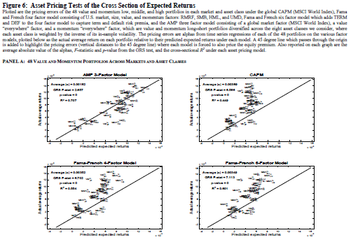
Figure 6: Asset Pricing Tests of the Cross Section of Expected Returns (28:31)

Next, the authors perform this same regression using other common asset pricing models, such as the CAPM and the Fama-French 4-factor and 6-factor models.  They find their AMP 3-factor model (at an R^2 of 0.71) does a better job at predicting the actual returns to the portfolios than do the other common pricing models.  They also perform this for US assets only, using the global factor loadings; they find that the Fama-French 4-factor and 6-factor models do a better job at predicting the portfolio returns than does the AMP 3-factor model, but this is because the AMP model is using global data to form the regression, while the Fama-French models are using US data to form the regressions.  It makes sense that US data does better at predicting US returns; however, the authors want to emphasize how well the global data in the AMP model predicts returns of US assets, further exhibiting the interconnectedness of the markets and factors.

Table 5: Cross-Sectional Asset Pricing Tests of Global Value and Momentum Strategies (31:58)

Next, the authors want to see how various economic indicators explain the returns of each of the 48 portfolios in this study.  They find that liquidity risk is significantly positively related to the returns of the portfolios when regressed along, and term risk and default risk are also significantly related; however, when those risk measures are combined in a regression, the liquidity risk subsumes the term and default risk; and further, when value and momentum factors are included in the regression, the liquidity risk is subsumed by those factors.  As such, the value and momentum premiums may be capturing liquidity risk.

Next, the authors explore funding and market liquidity separately, and they find that the funding liquidity is the factor that has the most influence on the returns (and not necessarily market liquidity); in both cases, however, the value and momentum factors subsume the liquidity risk measure.

Table 6: Time Series Asset Pricing Tests of Global Value and Momentum Strategies (34:42)

Next, the authors explore the regressions of several asset pricing models (i.e., the CAPM, Fama-French models, macroeconomic models, and APM 3-factor model).  They find the APM 3-factor model best explains the cross-section of returns (i.e., it has the highest R^2, the lowest alpha, and the lowest F-stat).  This means that a regression with the global zero-cost value, zero-cost momentum, and market factor do a good job of explaining the returns to these portfolios.

Next, they use the Fama-French 25 value / 25 momentum portfolios for forming the regression. As we saw in a previous table, the Fama-French 6-factor model does a better job of explaining the US returns because it uses US data in forming the regression; but the AMP 3-factor model (global market, value and momentum) still does a good job of explaining the returns.

Next, the authors explore how well the models can explain hedge fund returns (given the increased use by hedge funds in using factor-based portfolios).  They find the AMP 3-factor model does the best at explaining the hedge-fund returns. 

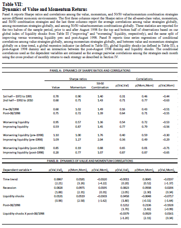
Table 7: Dynamics of Value and Momentum Returns (40:07)

Finally, given the success of these value and momentum strategies, the authors look at the performance of the strategies over different time periods ('72-'91 and '92-'10).  They find that the returns and sharpe ratios of the value and momentum strategies have decreased in the more recent period than the former period; however, the returns of the combined momentum/value strategy has remained constant across both periods.  The correlations within the value and momentum strategies have significantly increased from the prior period to the more recent period; however, the correlations between value and momentum strategies have become more negative.

Abstract

We study the returns to value and momentum strategies jointly across eight diverse markets and asset classes. Finding consistent value and momentum premia in every asset class, we further find strong common factor structure among their returns. Value and momentum are more positively correlated across asset classes than passive exposures to the asset classes themselves. However, value and momentum are negatively correlated both within and across asset classes. Our results indicate the presence of common global risks that we characterize with a three factor model. Global funding liquidity risk is a partial source of these patterns, which are identifiable only when examining value and momentum simultaneously across markets. Our findings present a challenge to existing behavioral, institutional, and rational asset pricing theories that largely focus on U.S. equities.

Suggested Citation: 

Asness, Cliff S. and Moskowitz, Tobias J. and Pedersen, Lasse Heje, Value and Momentum Everywhere (June 1, 2012). Chicago Booth Research Paper No. 12-53; Fama-Miller Working Paper. Available at SSRN: https://ssrn.com/abstract=2174501 or http://dx.doi.org/10.2139/ssrn.2174501